Euluer-bernouli beam theory

 Euler–Bernoulli beam theory (also known as engineer's beam theory or classical beam theory)^[1] is a simplification of the linear theory of elasticity which provides a means of calculating the load-carrying and deflection characteristics of beams. It covers the case corresponding to small deflections of a beam that is subjected to lateral loads only. By ignoring the effects of shear deformation and rotatory inertia, it is thus a special case of Timoshenko beam theory. It was first enunciated circa 1750,^[2] but was not applied on a large scale until the development of the Eiffel Tower and the Ferris wheel in the late 19th century. Following these successful demonstrations, it quickly became a cornerstone of engineering and an enabler of the Second Industrial Revolution.

This vibrating glass beam may be modeled as a cantilever beam with acceleration, variable linear density, variable section modulus, some kind of dissipation, springy end loading, and possibly a point mass at the free end.

Additional mathematical models have been developed, such as plate theory, but the simplicity of beam theory makes it an important tool in the sciences, especially structural and mechanical engineering.

HistoryEdit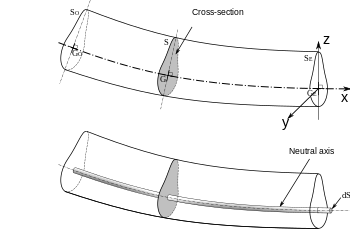

Schematic of cross-section of a bent beam showing the neutral axis.

Prevailing consensus is that Galileo Galilei made the first attempts at developing a theory of beams, but recent studies argue that Leonardo da Vinci was the first to make the crucial observations. Da Vinci lacked Hooke's law and calculus to complete the theory, whereas Galileo was held back by an incorrect assumption he made.^[3]

The Bernoulli beam is named after Jacob Bernoulli, who made the significant discoveries. Leonhard Euler and Daniel Bernoulli were the first to put together a useful theory circa 1750.^[4]

Static beam equationEdit

The Euler–Bernoulli equation describes the relationship between the beam's deflection and the applied load:^[5]

${\displaystyle {\frac {\mathrm {d} ^{2}}{\mathrm {d} x^{2}}}\left(EI{\frac {\mathrm {d} ^{2}w}{\mathrm {d} x^{2}}}\right)=q\,}$

The curve ${\displaystyle w(x)}$ describes the deflection of the beam in the ${\displaystyle z}$ direction at some position ${\displaystyle x}$ (recall that the beam is modeled as a one-dimensional object). ${\displaystyle q}$ is a distributed load, in other words a force per unit length (analogous to pressure being a force per area); it may be a function of ${\displaystyle x}$, ${\displaystyle w}$, or other variables. ${\displaystyle E}$ is the elastic modulus and ${\displaystyle I}$ is the second moment of area of the beam's cross section. ${\displaystyle I}$ must be calculated with respect to the axis which is perpendicular to the applied loading and which passes through the centroid of the cross section.^{[N 1]} Explicitly, for a beam whose axis is oriented along ${\displaystyle x}$ with a loading along ${\displaystyle z}$, the beam's cross section is in the ${\displaystyle yz}$ plane, and the relevant second moment of area is

${\displaystyle I=\iint z^{2}\;dy\;dz,}$

where it is assumed that the centroid of the cross section occurs at ${\displaystyle y=z=0}$.

Often, the product ${\displaystyle EI}$ (known as the flexural rigidity) is a constant, so that

${\displaystyle EI{\frac {\mathrm {d} ^{4}w}{\mathrm {d} x^{4}}}=q(x).\,}$

This equation, describing the deflection of a uniform, static beam, is used widely in engineering practice. Tabulated expressions for the deflection ${\displaystyle w}$ for common beam configurations can be found in engineering handbooks. For more complicated situations, the deflection can be determined by solving the Euler–Bernoulli equation using techniques such as "direct integration", "Macaulay's method", "moment area method, "conjugate beam method", "the principle of virtual work", "Castigliano's method", "flexibility method", "slope deflection method", "moment distribution method", or "direct stiffness method".

Sign conventions are defined here since different conventions can be found in the literature.^[5] In this article, a right-handed coordinate system is used with the ${\displaystyle x}$ axis to the right, the ${\displaystyle z}$ axis pointing upwards, and the ${\displaystyle y}$ axis pointing into the figure. The sign of the bending moment ${\displaystyle M}$ is taken as positive when the torque vector associated with the bending moment on the right hand side of the section is in the positive ${\displaystyle y}$ direction, that is, a positive value of ${\displaystyle M}$ produces compressive stress at the bottom surface. With this choice of bending moment sign convention, in order to have ${\displaystyle dM=Qdx}$, it is necessary that the shear force ${\displaystyle Q}$ acting on the right side of the section be positive in the ${\displaystyle z}$ direction so as to achieve static equilibrium of moments. If the loading intensity ${\displaystyle q}$ is taken positive in the positive ${\displaystyle z}$ direction, then ${\displaystyle dQ=-qdx}$ is necessary for force equilibrium.

Successive derivatives of the deflection ${\displaystyle w}$ have important physical meanings: ${\displaystyle dw/dx}$ is the slope of the beam, which is the anti-clockwise angle of rotation about the ${\displaystyle y}$-axis in the limit of small displacements;

${\displaystyle M=-EI{\frac {d^{2}w}{dx^{2}}}}$

is the bending moment in the beam; and

${\displaystyle Q=-{\frac {d}{dx}}\left(EI{\frac {d^{2}w}{dx^{2}}}\right)}$

is the shear force in the beam.

Bending of an Euler–Bernoulli beam. Each cross section of the beam is at 90 degrees to the neutral axis.

The stresses in a beam can be calculated from the above expressions after the deflection due to a given load has been determined.

Derivation of the bending equationEdit

Because of the fundamental importance of the bending moment equation in engineering, we will provide a short derivation. We change to polar coordinates. The length of the neutral axis in the figure is ${\displaystyle \rho d\theta .}$ The length of a fiber with a radial distance ${\displaystyle z}$ below the neutral axis is ${\displaystyle (\rho +z)d\theta .}$ Therefore, the strain of this fiber is

${\displaystyle {\frac {\left(\rho +z-\rho \right)\ d\theta }{\rho \ d\theta }}={\frac {z}{\rho }}.}$

The stress of this fiber is ${\displaystyle E{\dfrac {z}{\rho }}}$ where ${\displaystyle E}$ is the elastic modulus in accordance with Hooke's Law. The differential force vector, ${\displaystyle d\mathbf {F} ,}$ resulting from this stress is given by,

${\displaystyle d\mathbf {F} =E{\frac {z}{\rho }}dA\mathbf {e_{x}} .}$

This is the differential force vector exerted on the right hand side of the section shown in the figure. We know that it is in the ${\displaystyle \mathbf {e_{x}} }$ direction since the figure clearly shows that the fibers in the lower half are in tension. ${\displaystyle dA}$ is the differential element of area at the location of the fiber. The differential bending moment vector, ${\displaystyle d\mathbf {M} }$ associated with ${\displaystyle d\mathbf {F} }$ is given by

${\displaystyle d\mathbf {M} =-z\mathbf {e_{z}} \times d\mathbf {F} =-\mathbf {e_{y}} E{\frac {z^{2}}{\rho }}dA.}$

This expression is valid for the fibers in the lower half of the beam. The expression for the fibers in the upper half of the beam will be similar except that the moment arm vector will be in the positive ${\displaystyle z}$ direction and the force vector will be in the ${\displaystyle -x}$ direction since the upper fibers are in compression. But the resulting bending moment vector will still be in the ${\displaystyle -y}$ direction since ${\displaystyle \mathbf {e_{z}} \times -\mathbf {e_{x}} =-\mathbf {e_{y}} .}$ Therefore, we integrate over the entire cross section of the beam and get for ${\displaystyle \mathbf {M} }$ the bending moment vector exerted on the right cross section of the beam the expression

${\displaystyle \mathbf {M} =\int d\mathbf {M} =-\mathbf {e_{y}} {\frac {E}{\rho }}\int {z^{2}}\ dA=-\mathbf {e_{y}} {\frac {EI}{\rho }},}$

where ${\displaystyle I}$ is the second moment of area. From calculus, we know that when ${\displaystyle {\dfrac {dw}{dx}}}$ is small, as it is for an Euler–Bernoulli beam, we can make the approximation ${\displaystyle {\dfrac {1}{\rho }}\simeq {\dfrac {d^{2}w}{dx^{2}}}}$, where ${\displaystyle \rho }$ is the radius of curvature. Therefore,

${\displaystyle \mathbf {M} =-\mathbf {e_{y}} EI{d^{2}w \over dx^{2}}.}$

This vector equation can be separated in the bending unit vector definition (${\displaystyle M}$ is oriented as ${\displaystyle \mathbf {e_{y}} }$), and in the bending equation:

${\displaystyle M=-EI{d^{2}w \over dx^{2}}.}$

Dynamic beam equationEdit

Finite element method model of a vibration of a wide-flange beam (I-beam).

The dynamic beam equation is the Euler–Lagrange equation for the following action

${\displaystyle S=\int _{t_{1}}^{t_{2}}\int _{0}^{L}\left[{\frac {1}{2}}\mu \left({\frac {\partial w}{\partial t}}\right)^{2}-{\frac {1}{2}}EI\left({\frac {\partial ^{2}w}{\partial x^{2}}}\right)^{2}+q(x)w(x,t)\right]dxdt.}$

The first term represents the kinetic energy where ${\displaystyle \mu }$ is the mass per unit length, the second term represents the potential energy due to internal forces (when considered with a negative sign), and the third term represents the potential energy due to the external load ${\displaystyle q(x)}$. The Euler–Lagrange equation is used to determine the function that minimizes the functional ${\displaystyle S}$. For a dynamic Euler–Bernoulli beam, the Euler–Lagrange equation is

${\displaystyle {\cfrac {\partial ^{2}}{\partial x^{2}}}\left(EI{\cfrac {\partial ^{2}w}{\partial x^{2}}}\right)=-\mu {\cfrac {\partial ^{2}w}{\partial t^{2}}}+q(x).}$

Derivation of Euler–Lagrange equation for beams

Since the Lagrangian is ${\displaystyle {\mathcal {L}}:={\tfrac {1}{2}}\mu \left({\frac {\partial w}{\partial t}}\right)^{2}-{\tfrac {1}{2}}EI\left({\frac {\partial ^{2}w}{\partial x^{2}}}\right)^{2}+q(x)w(x,t)={\tfrac {\mu }{2}}{\dot {w}}^{2}-{\tfrac {EI}{2}}w_{xx}^{2}+qw\equiv {\mathcal {L}}(x,t,w,{\dot {w}},w_{xx})}$ the corresponding Euler–Lagrange equation is ${\displaystyle {\cfrac {\partial {\mathcal {L}}}{\partial w}}-{\frac {\partial }{\partial t}}\left({\frac {\partial {\mathcal {L}}}{\partial {\dot {w}}}}\right)+{\frac {\partial ^{2}}{\partial x^{2}}}\left({\frac {\partial {\mathcal {L}}}{\partial w_{xx}}}\right)=0}$ Now, ${\displaystyle {\cfrac {\partial {\mathcal {L}}}{\partial w}}=q~;~~{\frac {\partial {\mathcal {L}}}{\partial {\dot {w}}}}=\mu {\dot {w}}~;~~{\frac {\partial {\mathcal {L}}}{\partial w_{xx}}}=-EIw_{xx}~.}$ Plugging into the Euler–Lagrange equation gives ${\displaystyle q-\mu {\ddot {w}}-(EIw_{xx})_{xx}=0}$ or, ${\displaystyle {\cfrac {\partial ^{2}}{\partial x^{2}}}\left(EI{\cfrac {\partial ^{2}w}{\partial x^{2}}}\right)=-\mu {\cfrac {\partial ^{2}w}{\partial t^{2}}}+q}$ which is the governing equation for the dynamics of an Euler–Bernoulli beam.

When the beam is homogeneous, ${\displaystyle E}$ and ${\displaystyle I}$ are independent of ${\displaystyle x}$, and the beam equation is simpler:

${\displaystyle EI{\cfrac {\partial ^{4}w}{\partial x^{4}}}=-\mu {\cfrac {\partial ^{2}w}{\partial t^{2}}}+q\,.}$

Free vibrationEdit

In the absence of a transverse load, ${\displaystyle q}$, we have the free vibration equation. This equation can be solved using a Fourier decomposition of the displacement into the sum of harmonic vibrations of the form

${\displaystyle w(x,t)={\text{Re}}[{\hat {w}}(x)~e^{-i\omega t}]}$

where ${\displaystyle \omega }$ is the frequency of vibration. Then, for each value of frequency, we can solve an ordinary differential equation

${\displaystyle EI~{\cfrac {\mathrm {d} ^{4}{\hat {w}}}{\mathrm {d} x^{4}}}-\mu \omega ^{2}{\hat {w}}=0\,.}$ 

The general solution of the above equation is

${\displaystyle {\hat {w}}=A_{1}\cosh(\beta x)+A_{2}\sinh(\beta x)+A_{3}\cos(\beta x)+A_{4}\sin(\beta x)\quad {\text{with}}\quad \beta :=\left({\frac {\mu \omega ^{2}}{EI}}\right)^{1/4}}$ 

where ${\displaystyle A_{1},A_{2},A_{3},A_{4}}$  are constants. These constants are unique for a given set of boundary conditions. However, the solution for the displacement is not unique and depends on the frequency. These solutions are typically written as

${\displaystyle {\hat {w}}_{n}=A_{1}\cosh(\beta _{n}x)+A_{2}\sinh(\beta _{n}x)+A_{3}\cos(\beta _{n}x)+A_{4}\sin(\beta _{n}x)\quad {\text{with}}\quad \beta _{n}:=\left({\frac {\mu \omega _{n}^{2}}{EI}}\right)^{1/4}\,.}$ 

The quantities ${\displaystyle \omega _{n}}$  are called the natural frequencies of the beam. Each of the displacement solutions is called a mode, and the shape of the displacement curve is called a mode shape.

Example: Cantilevered beamEdit

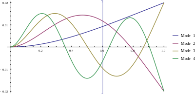
Mode shapes for the first four modes of a vibrating cantilever beam.

The boundary conditions for a cantilevered beam of length ${\displaystyle L}$ (fixed at ${\displaystyle x=0}$) are

${\displaystyle {\begin{aligned}&{\hat {w}}_{n}=0~,~~{\frac {d{\hat {w}}_{n}}{dx}}=0\quad {\text{at}}~~x=0\\&{\frac {d^{2}{\hat {w}}_{n}}{dx^{2}}}=0~,~~{\frac {d^{3}{\hat {w}}_{n}}{dx^{3}}}=0\quad {\text{at}}~~x=L\,.\end{aligned}}}$

If we apply these conditions, non-trivial solutions are found to exist only if ${\displaystyle \cosh(\beta _{n}L)\,\cos(\beta _{n}L)+1=0\,.}$ This nonlinear equation can be solved numerically. The first four roots are ${\displaystyle \beta _{1}L=0.596864\pi }$, ${\displaystyle \beta _{2}L=1.49418\pi }$, ${\displaystyle \beta _{3}L=2.50025\pi }$, and ${\displaystyle \beta _{4}L=3.49999\pi }$.

The corresponding natural frequencies of vibration are

${\displaystyle \omega _{1}=\beta _{1}^{2}{\sqrt {\frac {EI}{\mu }}}={\frac {3.5160}{L^{2}}}{\sqrt {\frac {EI}{\mu }}}~,~~\dots }$

The boundary conditions can also be used to determine the mode shapes from the solution for the displacement:

${\displaystyle {\hat {w}}_{n}=A_{1}\left[(\cosh \beta _{n}x-\cos \beta _{n}x)+{\frac {\cos \beta _{n}L+\cosh \beta _{n}L}{\sin \beta _{n}L+\sinh \beta _{n}L}}(\sin \beta _{n}x-\sinh \beta _{n}x)\right]}$

The unknown constant (actually constants as there is one for each ${\displaystyle n}$), ${\displaystyle A_{1}}$, which in general is complex, is determined by the initial conditions at ${\displaystyle t=0}$ on the velocity and displacements of the beam. Typically a value of ${\displaystyle A_{1}=1}$ is used when plotting mode shapes. Solutions to the undampened forced problem have unbounded displacements when the driving frequency matches a natural frequency ${\displaystyle \omega _{n}}$, i.e., the beam can resonate. The natural frequencies of a beam therefore correspond to the frequencies at which resonance can occur.

Example: free–free (unsupported) beamEdit

The first four modes of a vibrating free–free Euler-Bernoulli beam.

A free–free beam is a beam without any supports.^[6] The boundary conditions for a free–free beam of length ${\displaystyle L}$ extending from ${\displaystyle x=0}$ to ${\displaystyle x=L}$ are given by:

${\displaystyle {\frac {d^{2}{\hat {w}}_{n}}{dx^{2}}}=0~,~~{\frac {d^{3}{\hat {w}}_{n}}{dx^{3}}}=0\quad {\text{at}}~~x=0\,{\text{and}}\,x=L\,.}$

If we apply these conditions, non-trivial solutions are found to exist only if

${\displaystyle \cosh(\beta _{n}L)\,\cos(\beta _{n}L)-1=0\,.}$

This nonlinear equation can be solved numerically. The first four roots are ${\displaystyle \beta _{1}L=1.50562\pi }$, ${\displaystyle \beta _{2}L=2.49975\pi }$, ${\displaystyle \beta _{3}L=3.50001\pi }$, and ${\displaystyle \beta _{4}L=4.50000\pi }$.

The corresponding natural frequencies of vibration are:

${\displaystyle \omega _{1}=\beta _{1}^{2}{\sqrt {\frac {EI}{\mu }}}={\frac {22.3733}{L^{2}}}{\sqrt {\frac {EI}{\mu }}}~,~~\dots }$

The boundary conditions can also be used to determine the mode shapes from the solution for the displacement:

${\displaystyle {\hat {w}}_{n}=A_{1}{\Bigl [}(\cos \beta _{n}x+\cosh \beta _{n}x)-{\frac {\cos \beta _{n}L-\cosh \beta _{n}L}{\sin \beta _{n}L-\sinh \beta _{n}L}}(\sin \beta _{n}x+\sinh \beta _{n}x){\Bigr ]}}$

As with the cantilevered beam, the unknown constants are determined by the initial conditions at ${\displaystyle t=0}$ on the velocity and displacements of the beam. Also, solutions to the undampened forced problem have unbounded displacements when the driving frequency matches a natural frequency ${\displaystyle \omega _{n}}$.

StressEdit

Besides deflection, the beam equation describes forces and moments and can thus be used to describe stresses. For this reason, the Euler–Bernoulli beam equation is widely used in engineering, especially civil and mechanical, to determine the strength (as well as deflection) of beams under bending.

Both the bending moment and the shear force cause stresses in the beam. The stress due to shear force is maximum along the neutral axis of the beam (when the width of the beam, t, is constant along the cross section of the beam; otherwise an integral involving the first moment and the beam's width needs to be evaluated for the particular cross section), and the maximum tensile stress is at either the top or bottom surfaces. Thus the maximum principal stress in the beam may be neither at the surface nor at the center but in some general area. However, shear force stresses are negligible in comparison to bending moment stresses in all but the stockiest of beams as well as the fact that stress concentrations commonly occur at surfaces, meaning that the maximum stress in a beam is likely to be at the surface.

Simple or symmetrical bendingEdit

Element of a bent beam: the fibers form concentric arcs, the top fibers are compressed and bottom fibers stretched.

For beam cross-sections that are symmetrical about a plane perpendicular to the neutral plane, it can be shown that the tensile stress experienced by the beam may be expressed as:

${\displaystyle \sigma ={\frac {Mz}{I}}=-zE~{\frac {\mathrm {d} ^{2}w}{\mathrm {d} x^{2}}}.\,}$

Here, ${\displaystyle z}$ is the distance from the neutral axis to a point of interest; and ${\displaystyle M}$ is the bending moment. Note that this equation implies that pure bending (of positive sign) will cause zero stress at the neutral axis, positive (tensile) stress at the "top" of the beam, and negative (compressive) stress at the bottom of the beam; and also implies that the maximum stress will be at the top surface and the minimum at the bottom. This bending stress may be superimposed with axially applied stresses, which will cause a shift in the neutral (zero stress) axis.

Maximum stresses at a cross-sectionEdit

Quantities used in the definition of the section modulus of a beam.

The maximum tensile stress at a cross-section is at the location ${\displaystyle z=c_{1}}$ and the maximum compressive stress is at the location ${\displaystyle z=-c_{2}}$ where the height of the cross-section is ${\displaystyle h=c_{1}+c_{2}}$. These stresses are

${\displaystyle \sigma _{1}={\cfrac {Mc_{1}}{I}}={\cfrac {M}{S_{1}}}~;~~\sigma _{2}=-{\cfrac {Mc_{2}}{I}}=-{\cfrac {M}{S_{2}}}}$

The quantities ${\displaystyle S_{1},S_{2}}$ are the section moduli^[5] and are defined as

${\displaystyle S_{1}={\cfrac {I}{c_{1}}}~;~~S_{2}={\cfrac {I}{c_{2}}}}$

The section modulus combines all the important geometric information about a beam's section into one quantity. For the case where a beam is doubly symmetric, ${\displaystyle c_{1}=c_{2}}$ and we have one section modulus ${\displaystyle S=I/c}$.

Strain in an Euler–Bernoulli beamEdit

We need an expression for the strain in terms of the deflection of the neutral surface to relate the stresses in an Euler–Bernoulli beam to the deflection. To obtain that expression we use the assumption that normals to the neutral surface remain normal during the deformation and that deflections are small. These assumptions imply that the beam bends into an arc of a circle of radius ${\displaystyle \rho }$ (see Figure 1) and that the neutral surface does not change in length during the deformation.^[5]

Let ${\displaystyle \mathrm {d} x}$ be the length of an element of the neutral surface in the undeformed state. For small deflections, the element does not change its length after bending but deforms into an arc of a circle of radius ${\displaystyle \rho }$. If ${\displaystyle \mathrm {d} \theta }$ is the angle subtended by this arc, then ${\displaystyle \mathrm {d} x=\rho ~\mathrm {d} \theta }$.

Let us now consider another segment of the element at a distance ${\displaystyle z}$ above the neutral surface. The initial length of this element is ${\displaystyle \mathrm {d} x}$. However, after bending, the length of the element becomes ${\displaystyle \mathrm {d} x'=(\rho -z)~\mathrm {d} \theta =\mathrm {d} x-z~\mathrm {d} \theta }$. The strain in that segment of the beam is given by

${\displaystyle \varepsilon _{x}={\cfrac {\mathrm {d} x'-\mathrm {d} x}{\mathrm {d} x}}=-{\cfrac {z}{\rho }}=-\kappa ~z}$

where ${\displaystyle \kappa }$ is the curvature of the beam. This gives us the axial strain in the beam as a function of distance from the neutral surface. However, we still need to find a relation between the radius of curvature and the beam deflection ${\displaystyle w}$.

Relation between curvature and beam deflectionEdit

Let P be a point on the neutral surface of the beam at a distance ${\displaystyle x}$ from the origin of the ${\displaystyle (x,z)}$ coordinate system. The slope of the beam is approximately equal to the angle made by the neutral surface with the ${\displaystyle x}$-axis for the small angles encountered in beam theory. Therefore, with this approximation,

${\displaystyle \theta (x)={\cfrac {\mathrm {d} w}{\mathrm {d} x}}}$

Therefore, for an infinitesimal element ${\displaystyle \mathrm {d} x}$, the relation ${\displaystyle \mathrm {d} x=\rho ~\mathrm {d} \theta }$ can be written as

${\displaystyle {\cfrac {1}{\rho }}={\cfrac {\mathrm {d} \theta }{\mathrm {d} x}}={\cfrac {\mathrm {d} ^{2}w}{\mathrm {d} x^{2}}}=\kappa }$

Hence the strain in the beam may be expressed as

${\displaystyle \varepsilon _{x}=-z\kappa }$

Stress-strain relationsEdit

For a homogeneous isotropic linear elastic material, the stress is related to the strain by ${\displaystyle \sigma =E\varepsilon }$, where ${\displaystyle E}$ is the Young's modulus. Hence the stress in an Euler–Bernoulli beam is given by

${\displaystyle \sigma _{x}=-zE{\cfrac {\mathrm {d} ^{2}w}{\mathrm {d} x^{2}}}}$

Note that the above relation, when compared with the relation between the axial stress and the bending moment, leads to

${\displaystyle M=-EI{\cfrac {\mathrm {d} ^{2}w}{\mathrm {d} x^{2}}}}$

Since the shear force is given by ${\displaystyle Q=\mathrm {d} M/\mathrm {d} x}$, we also have

${\displaystyle Q=-EI{\cfrac {\mathrm {d} ^{3}w}{\mathrm {d} x^{3}}}}$