Contact mechanic

 Contact mechanics is the study of the deformation of solids that touch each other at one or more points.^[1][2] A central distinction in contact mechanics is between stresses acting perpendicular to the contacting bodies' surfaces (known as the normal direction) and frictional stresses acting tangentially between the surfaces. This page focuses mainly on the normal direction, i.e. on frictionless contact mechanics. Frictional contact mechanics is discussed separately. Normal stresses are caused by applied forces and by the adhesion present on surfaces in close contact even if they are clean and dry.

Stresses in a contact area loaded simultaneously with a normal and a tangential force. Stresses were made visible using photoelasticity.

Contact mechanics is part of mechanical engineering. The physical and mathematical formulation of the subject is built upon the mechanics of materials and continuum mechanics and focuses on computations involving elastic, viscoelastic, and plastic bodies in static or dynamic contact. Contact mechanics provides necessary information for the safe and energy efficient design of technical systems and for the study of tribology, contact stiffness, electrical contact resistance and indentation hardness. Principles of contacts mechanics are implemented towards applications such as locomotive wheel-rail contact, coupling devices, braking systems, tires, bearings, combustion engines, mechanical linkages, gasket seals, metalworking, metal forming, ultrasonic welding, electrical contacts, and many others. Current challenges faced in the field may include stress analysis of contact and coupling members and the influence of lubrication and material design on friction and wear. Applications of contact mechanics further extend into the micro- and nanotechnological realm.

The original work in contact mechanics dates back to 1881 with the publication of the paper "On the contact of elastic solids"^[3] ("Ueber die Berührung fester elastischer Körper") by Heinrich Hertz. Hertz was attempting to understand how the optical properties of multiple, stacked lenses might change with the force holding them together. Hertzian contact stress refers to the localized stresses that develop as two curved surfaces come in contact and deform slightly under the imposed loads. This amount of deformation is dependent on the modulus of elasticity of the material in contact. It gives the contact stress as a function of the normal contact force, the radii of curvature of both bodies and the modulus of elasticity of both bodies. Hertzian contact stress forms the foundation for the equations for load bearing capabilities and fatigue life in bearings, gears, and any other bodies where two surfaces are in contact.

HistoryEdit

When a sphere is pressed against an elastic material, the contact area increases.

Classical contact mechanics is most notably associated with Heinrich Hertz.^[3][4] In 1882, Hertz solved the contact problem of two elastic bodies with curved surfaces. This still-relevant classical solution provides a foundation for modern problems in contact mechanics. For example, in mechanical engineering and tribology, Hertzian contact stress is a description of the stress within mating parts. The Hertzian contact stress usually refers to the stress close to the area of contact between two spheres of different radii.

It was not until nearly one hundred years later that Johnson, Kendall, and Roberts found a similar solution for the case of adhesive contact.^[5] This theory was rejected by Boris Derjaguin and co-workers^[6] who proposed a different theory of adhesion^[7] in the 1970s. The Derjaguin model came to be known as the DMT (after Derjaguin, Muller and Toporov) model,^[7] and the Johnson et al. model came to be known as the JKR (after Johnson, Kendall and Roberts) model for adhesive elastic contact. This rejection proved to be instrumental in the development of the Tabor^[8] and later Maugis^[6][9] parameters that quantify which contact model (of the JKR and DMT models) represent adhesive contact better for specific materials.

Further advancement in the field of contact mechanics in the mid-twentieth century may be attributed to names such as Bowden and Tabor. Bowden and Tabor were the first to emphasize the importance of surface roughness for bodies in contact.^[10][11] Through investigation of the surface roughness, the true contact area between friction partners is found to be less than the apparent contact area. Such understanding also drastically changed the direction of undertakings in tribology. The works of Bowden and Tabor yielded several theories in contact mechanics of rough surfaces.

The contributions of Archard (1957)^[12] must also be mentioned in discussion of pioneering works in this field. Archard concluded that, even for rough elastic surfaces, the contact area is approximately proportional to the normal force. Further important insights along these lines were provided by Greenwood and Williamson (1966),^[13] Bush (1975),^[14] and Persson (2002).^[15] The main findings of these works were that the true contact surface in rough materials is generally proportional to the normal force, while the parameters of individual micro-contacts (i.e., pressure, size of the micro-contact) are only weakly dependent upon the load.

Classical solutions for non-adhesive elastic contactEdit

The theory of contact between elastic bodies can be used to find contact areas and indentation depths for simple geometries. Some commonly used solutions are listed below. The theory used to compute these solutions is discussed later in the article. Solutions for multitude of other technically relevant shapes, e.g. the truncated cone, the worn sphere, rough profiles, hollow cylinders, etc. can be found in ^[16]

Contact between a sphere and a half-spaceEdit

Contact of an elastic sphere with an elastic half-space

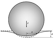
An elastic sphere of radius ${\displaystyle R}$ indents an elastic half-space where total deformation is ${\displaystyle d}$, causing a contact area of radius

${\displaystyle a={\sqrt {Rd}}}$

The applied force ${\displaystyle F}$ is related to the displacement ${\displaystyle d}$ by ^[4]

${\displaystyle F={\frac {4}{3}}E^{*}R^{\frac {1}{2}}d^{\frac {3}{2}}}$

where

${\displaystyle {\frac {1}{E^{*}}}={\frac {1-\nu _{1}^{2}}{E_{1}}}+{\frac {1-\nu _{2}^{2}}{E_{2}}}}$

and ${\displaystyle E_{1}}$,${\displaystyle E_{2}}$ are the elastic moduli and ${\displaystyle \nu _{1}}$,${\displaystyle \nu _{2}}$ the Poisson's ratios associated with each body.

The distribution of normal pressure in the contact area as a function of distance from the center of the circle is^[1]

${\displaystyle p(r)=p_{0}\left(1-{\frac {r^{2}}{a^{2}}}\right)^{\frac {1}{2}}}$

where ${\displaystyle p_{0}}$ is the maximum contact pressure given by

${\displaystyle p_{0}={\frac {3F}{2\pi a^{2}}}={\frac {1}{\pi }}\left({\frac {6F{E^{*}}^{2}}{R^{2}}}\right)^{\frac {1}{3}}}$

The radius of the circle is related to the applied load ${\displaystyle F}$ by the equation

${\displaystyle a^{3}={\cfrac {3FR}{4E^{*}}}}$

The total deformation ${\displaystyle d}$ is related to the maximum contact pressure by

${\displaystyle d={\frac {a^{2}}{R}}=\left({\frac {9F^{2}}{16{E^{*}}^{2}R}}\right)^{\frac {1}{3}}}$

The maximum shear stress occurs in the interior at ${\displaystyle z\approx 0.49a}$ for ${\displaystyle \nu =0.33}$.

Contact between two spheresEdit

Contact between two spheres.

Contact between two crossed cylinders of equal radius.

For contact between two spheres of radii ${\displaystyle R_{1}}$ and ${\displaystyle R_{2}}$, the area of contact is a circle of radius ${\displaystyle a}$. The equations are the same as for a sphere in contact with a half plane except that the effective radius ${\displaystyle R}$ is defined as ^[4]

${\displaystyle {\frac {1}{R}}={\frac {1}{R_{1}}}+{\frac {1}{R_{2}}}}$

Contact between two crossed cylinders of equal radius ${\displaystyle R}$Edit

This is equivalent to contact between a sphere of radius ${\displaystyle R}$ and a plane.

Contact between a rigid cylinder with flat end and an elastic half-spaceEdit

Contact between a rigid cylindrical indenter and an elastic half-space.

If a rigid cylinder is pressed into an elastic half-space, it creates a pressure distribution described by^[17]

${\displaystyle p(r)=p_{0}\left(1-{\frac {r^{2}}{R^{2}}}\right)^{-{\frac {1}{2}}}}$

where ${\displaystyle R}$ is the radius of the cylinder and

${\displaystyle p_{0}={\frac {1}{\pi }}E^{*}{\frac {d}{R}}}$

The relationship between the indentation depth and the normal force is given by

${\displaystyle F=2RE^{*}d}$

Contact between a rigid conical indenter and an elastic half-spaceEdit

Contact between a rigid conical indenter and an elastic half-space.

In the case of indentation of an elastic half-space of Young's modulus ${\displaystyle E}$ using a rigid conical indenter, the depth of the contact region ${\displaystyle \epsilon }$ and contact radius ${\displaystyle a}$ are related by^[17]

${\displaystyle \epsilon =a\tan(\theta )}$

with ${\displaystyle \theta }$ defined as the angle between the plane and the side surface of the cone. The total indentation depth ${\displaystyle d}$ is given by:

${\displaystyle d={\frac {\pi }{2}}\epsilon }$

The total force is

${\displaystyle F={\frac {\pi E}{2\left(1-\nu ^{2}\right)}}a^{2}\tan(\theta )={\frac {2E}{\pi \left(1-\nu ^{2}\right)}}{\frac {d^{2}}{\tan(\theta )}}}$

The pressure distribution is given by

${\displaystyle p\left(r\right)={\frac {Ed}{\pi a\left(1-\nu ^{2}\right)}}\ln \left({\frac {a}{r}}+{\sqrt {\left({\frac {a}{r}}\right)^{2}-1}}\right)={\frac {Ed}{\pi a\left(1-\nu ^{2}\right)}}\cosh ^{-1}\left({\frac {a}{r}}\right)}$

The stress has a logarithmic singularity at the tip of the cone.

Contact between two cylinders with parallel axesEdit

Contact between two cylinders with parallel axes

In contact between two cylinders with parallel axes, the force is linearly proportional to the length of cylinders L and to the indentation depth d:^[18]

${\displaystyle F\approx {\frac {\pi }{4}}E^{*}Ld}$

The radii of curvature are entirely absent from this relationship. The contact radius is described through the usual relationship

${\displaystyle a={\sqrt {Rd}}}$

with

${\displaystyle {\frac {1}{R}}={\frac {1}{R_{1}}}+{\frac {1}{R_{2}}}}$

as in contact between two spheres. The maximum pressure is equal to

${\displaystyle p_{0}=\left({\frac {E^{*}F}{\pi LR}}\right)^{\frac {1}{2}}}$

Bearing contactEdit

Main article: Bearing pressure

The contact in the case of bearings is often a contact between a convex surface (male cylinder or sphere) and a concave surface (female cylinder or sphere: bore or hemispherical cup).

The Method of Dimensionality ReductionEdit

Contact between a sphere and an elastic half-space and one-dimensional replaced model.

Some contact problems can be solved with the Method of Dimensionality Reduction (MDR). In this method, the initial three-dimensional system is replaced with a contact of a body with a linear elastic or viscoelastic foundation (see fig.). The properties of one-dimensional systems coincide exactly with those of the original three-dimensional system, if the form of the bodies is modified and the elements of the foundation are defined according to the rules of the MDR.^[19][20] MDR is based on the solution to axisymmetric contact problems first obtained by Ludwig Föppl (1941) and Gerhard Schubert (1942)^[21]

However, for exact analytical results, it is required that the contact problem is axisymmetric and the contacts are compact.

Hertzian theory of non-adhesive elastic contactEdit

The classical theory of contact focused primarily on non-adhesive contact where no tension force is allowed to occur within the contact area, i.e., contacting bodies can be separated without adhesion forces. Several analytical and numerical approaches have been used to solve contact problems that satisfy the no-adhesion condition. Complex forces and moments are transmitted between the bodies where they touch, so problems in contact mechanics can become quite sophisticated. In addition, the contact stresses are usually a nonlinear function of the deformation. To simplify the solution procedure, a frame of reference is usually defined in which the objects (possibly in motion relative to one another) are static. They interact through surface tractions (or pressures/stresses) at their interface.

As an example, consider two objects which meet at some surface ${\displaystyle S}$  in the (${\displaystyle x}$ ,${\displaystyle y}$ )-plane with the ${\displaystyle z}$ -axis assumed normal to the surface. One of the bodies will experience a normally-directed pressure distribution ${\displaystyle p_{z}=p(x,y)=q_{z}(x,y)}$ and in-plane surface traction distributions ${\displaystyle q_{x}=q_{x}(x,y)}$ and ${\displaystyle q_{y}=q_{y}(x,y)}$ over the region ${\displaystyle S}$. In terms of a Newtonian force balance, the forces:

${\displaystyle P_{z}=\int _{S}p(x,y)~\mathrm {d} A~;~~Q_{x}=\int _{S}q_{x}(x,y)~\mathrm {d} A~;~~Q_{y}=\int _{S}q_{y}(x,y)~\mathrm {d} A}$

must be equal and opposite to the forces established in the other body. The moments corresponding to these forces:

${\displaystyle M_{x}=\int _{S}y~q_{z}(x,y)~\mathrm {d} A~;~~M_{y}=\int _{S}-x~q_{z}(x,y)~\mathrm {d} A~;~~M_{z}=\int _{S}[x~q_{y}(x,y)-y~q_{x}(x,y)]~\mathrm {d} A}$

are also required to cancel between bodies so that they are kinematically immobile.

Assumptions in Hertzian theoryEdit

The following assumptions are made in determining the solutions of Hertzian contact problems:

• The strains are small and within the elastic limit.
• The surfaces are continuous and non-conforming (implying that the area of contact is much smaller than the characteristic dimensions of the contacting bodies).
• Each body can be considered an elastic half-space.
• The surfaces are frictionless.

Additional complications arise when some or all these assumptions are violated and such contact problems are usually called non-Hertzian.

Analytical solution techniquesEdit

Contact between two spheres.

Analytical solution methods for non-adhesive contact problem can be classified into two types based on the geometry of the area of contact.^[22] A conforming contact is one in which the two bodies touch at multiple points before any deformation takes place (i.e., they just "fit together"). A non-conforming contact is one in which the shapes of the bodies are dissimilar enough that, under zero load, they only touch at a point (or possibly along a line). In the non-conforming case, the contact area is small compared to the sizes of the objects and the stresses are highly concentrated in this area. Such a contact is called concentrated, otherwise it is called diversified.

A common approach in linear elasticity is to superpose a number of solutions each of which corresponds to a point load acting over the area of contact. For example, in the case of loading of a half-plane, the Flamant solution is often used as a starting point and then generalized to various shapes of the area of contact. The force and moment balances between the two bodies in contact act as additional constraints to the solution.

Point contact on a (2D) half-planeEdit

Main article: Flamant solution

Schematic of the loading on a plane by force P at a point (0, 0).

A starting point for solving contact problems is to understand the effect of a "point-load" applied to an isotropic, homogeneous, and linear elastic half-plane, shown in the figure to the right. The problem may be either plane stress or plane strain. This is a boundary value problem of linear elasticity subject to the traction boundary conditions:

${\displaystyle \sigma _{xz}(x,0)=0~;~~\sigma _{z}(x,z)=-P\delta (x,z)}$

where ${\displaystyle \delta (x,z)}$ is the Dirac delta function. The boundary conditions state that there are no shear stresses on the surface and a singular normal force P is applied at (0, 0). Applying these conditions to the governing equations of elasticity produces the result

${\displaystyle {\begin{aligned}\sigma _{xx}&=-{\frac {2P}{\pi }}{\frac {x^{2}z}{\left(x^{2}+z^{2}\right)^{2}}}\\\sigma _{zz}&=-{\frac {2P}{\pi }}{\frac {z^{3}}{\left(x^{2}+z^{2}\right)^{2}}}\\\sigma _{xz}&=-{\frac {2P}{\pi }}{\frac {xz^{2}}{\left(x^{2}+z^{2}\right)^{2}}}\end{aligned}}}$

for some point, ${\displaystyle (x,y)}$, in the half-plane. The circle shown in the figure indicates a surface on which the maximum shear stress is constant. From this stress field, the strain components and thus the displacements of all material points may be determined.

Line contact on a (2D) half-planeEdit

Normal loading over a region ${\displaystyle (a,b)}$Edit

Suppose, rather than a point load ${\displaystyle P}$, a distributed load ${\displaystyle p(x)}$ is applied to the surface instead, over the range ${\displaystyle a<x<b}$. The principle of linear superposition can be applied to determine the resulting stress field as the solution to the integral equations:

${\displaystyle {\begin{aligned}\sigma _{xx}&=-{\frac {2z}{\pi }}\int _{a}^{b}{\frac {p\left(x'\right)\left(x-x'\right)^{2}\,dx'}{\left[\left(x-x'\right)^{2}+z^{2}\right]^{2}}}~;~~\sigma _{zz}=-{\frac {2z^{3}}{\pi }}\int _{a}^{b}{\frac {p\left(x'\right)\,dx'}{\left[\left(x-x'\right)^{2}+z^{2}\right]^{2}}}\\[3pt]\sigma _{xz}&=-{\frac {2z^{2}}{\pi }}\int _{a}^{b}{\frac {p\left(x'\right)\left(x-x'\right)\,dx'}{\left[\left(x-x'\right)^{2}+z^{2}\right]^{2}}}\end{aligned}}}$

Shear loading over a region ${\displaystyle (a,b)}$Edit

The same principle applies for loading on the surface in the plane of the surface. These kinds of tractions would tend to arise as a result of friction. The solution is similar the above (for both singular loads ${\displaystyle Q}$ and distributed loads ${\displaystyle q(x)}$) but altered slightly:

${\displaystyle {\begin{aligned}\sigma _{xx}&=-{\frac {2}{\pi }}\int _{a}^{b}{\frac {q\left(x'\right)\left(x-x'\right)^{3}\,dx'}{\left[\left(x-x'\right)^{2}+z^{2}\right]^{2}}}~;~~\sigma _{zz}=-{\frac {2z^{2}}{\pi }}\int _{a}^{b}{\frac {q\left(x'\right)\left(x-x'\right)\,dx'}{\left[\left(x-x'\right)^{2}+z^{2}\right]^{2}}}\\[3pt]\sigma _{xz}&=-{\frac {2z}{\pi }}\int _{a}^{b}{\frac {q\left(x'\right)\left(x-x'\right)^{2}\,dx'}{\left[\left(x-x'\right)^{2}+z^{2}\right]^{2}}}\end{aligned}}}$

These results may themselves be superposed onto those given above for normal loading to deal with more complex loads.

Point contact on a (3D) half-spaceEdit

Analogously to the Flamant solution for the 2D half-plane, fundamental solutions are known for the linearly elastic 3D half-space as well. These were found by Boussinesq for a concentrated normal load and by Cerruti for a tangential load. See the section on this in Linear elasticity.

Numerical solution techniquesEdit

Distinctions between conforming and non-conforming contact do not have to be made when numerical solution schemes are employed to solve contact problems. These methods do not rely on further assumptions within the solution process since they base solely on the general formulation of the underlying equations.^{[23][24][25][26][27]} Besides the standard equations describing the deformation and motion of bodies two additional inequalities can be formulated. The first simply restricts the motion and deformation of the bodies by the assumption that no penetration can occur. Hence the gap ${\displaystyle h}$ between two bodies can only be positive or zero

${\displaystyle h\geq 0}$

where ${\displaystyle h=0}$ denotes contact. The second assumption in contact mechanics is related to the fact, that no tension force is allowed to occur within the contact area (contacting bodies can be lifted up without adhesion forces). This leads to an inequality which the stresses have to obey at the contact interface. It is formulated for the normal stress ${\displaystyle \sigma _{n}=\mathbf {t} \cdot \mathbf {n} }$.

At locations where there is contact between the surfaces the gap is zero, i.e. ${\displaystyle h=0}$, and there the normal stress is different than zero, indeed, ${\displaystyle \sigma _{n}<0}$. At locations where the surfaces are not in contact the normal stress is identical to zero; ${\displaystyle \sigma _{n}=0}$, while the gap is positive; i.e., ${\displaystyle h>0}$. This type of complementarity formulation can be expressed in the so-called Kuhn–Tucker form, viz.

${\displaystyle h\geq 0\,,\quad \sigma _{n}\leq 0\,,\quad \sigma _{n}\,h=0\,.}$

These conditions are valid in a general way. The mathematical formulation of the gap depends upon the kinematics of the underlying theory of the solid (e.g., linear or nonlinear solid in two- or three dimensions, beam or shell model). By restating the normal stress ${\displaystyle \sigma _{n}}$ in terms of the contact pressure, ${\displaystyle p}$; i.e., ${\displaystyle p=-\sigma _{n}}$ the Kuhn-Tucker problem can be restated as in standard complementarity form i.e.

$${\displaystyle h\geq 0\,,\quad p\geq 0\,,\quad p\,h=0\,.}$$

In the linear elastic case the gap can be formulated as

$${\displaystyle {h}=h_{0}+{g}+u,}$$

where ${\displaystyle h_{0}}$is the rigid body separation, ${\displaystyle g}$ is the geometry/topography of the contact (cylinder and roughness) and ${\displaystyle u}$ is the elastic deformation/deflection. If the contacting bodies are approximated as linear elastic half spaces, the Boussinesq-Cerruti integral equation solution can be applied to express the deformation (${\displaystyle u}$) as a function of the contact pressure (${\displaystyle p}$); i.e.,

$${\displaystyle u=\int _{\infty }^{\infty }K(x-s)p(s)ds,}$$

where

$${\displaystyle K(x-s)={\frac {2}{\pi E^{*}}}\ln |x-s|}$$

for line loading of an elastic half space and

$${\displaystyle K(x-s)={\frac {1}{\pi E^{*}}}{\frac {1}{\sqrt {\left(x_{1}-s_{1}\right)^{2}+\left(x_{2}-s_{2}\right)^{2}}}}}$$

for point loading of an elastic half-space.^[1]

After discretization the linear elastic contact mechanics problem can be stated in standard Linear Complementarity Problem (LCP) form.^[28]

${\displaystyle {\begin{aligned}\mathbf {h} &=\mathbf {h} _{0}+\mathbf {g} +\mathbf {Cp} ,\\\mathbf {h} \cdot \mathbf {p} &=0,\,\,\,\mathbf {p} \geq 0,\,\,\,\mathbf {h} \geq 0,\\\end{aligned}}}$

where ${\displaystyle \mathbf {C} }$ is a matrix, whose elements are so called influence coefficients relating the contact pressure and the deformation. The strict LCP formulation of the CM problem presented above, allows for direct application of well-established numerical solution techniques such as Lemke's pivoting algorithm. The Lemke algorithm has the advantage that it finds the numerically exact solution within a finite number of iterations. The MATLAB implementation presented by Almqvist et al. is one example that can be employed to solve the problem numerically. In addition, an example code for an LCP solution of a 2D linear elastic contact mechanics problem has also been made public at MATLAB file exchange by Almqvist et al.